Perform sensitivity analysis for published studies

For published studies, this command calculates (1) how much bias there must be in an estimate to nullify/sustain an inference; (2) the impact of an omitted variable necessary to nullify/sustain an inference for a regression coefficient. For a full description of the command’s usage and additional examples, please refer to our practical guide.

Usage

pkonfound(
  est_eff,
  std_err,
  n_obs,
  n_covariates = 1,
  alpha = 0.05,
  tails = 2,
  index = "RIR",
  nu = 0,
  n_treat = NULL,
  switch_trm = TRUE,
  model_type = "ols",
  a = NULL,
  b = NULL,
  c = NULL,
  d = NULL,
  two_by_two_table = NULL,
  test = "fisher",
  replace = "control",
  sdx = NA,
  sdy = NA,
  R2 = NA,
  far_bound = 0,
  eff_thr = NA,
  FR2max = 0,
  FR2max_multiplier = 1.3,
  to_return = "print",
  upper_bound = NULL,
  lower_bound = NULL,
  raw_treatment_success = NULL
)

Arguments

est_eff: the estimated effect (e.g., an unstandardized beta coefficient or a group mean difference).
std_err: the standard error of the estimate of the unstandardized regression coefficient.
n_obs: the number of observations in the sample.
n_covariates: the number of covariates in the regression model.
alpha: the probability of rejecting the null hypothesis (defaults to 0.05).
tails: integer indicating if the test is one-tailed (1) or two-tailed (2; defaults to 2).
index: specifies whether output is RIR or IT (impact threshold); defaults to "RIR".
nu: specifies the hypothesis to be tested; defaults to testing whether est_eff is significantly different from 0.
n_treat: the number of cases associated with the treatment condition (for logistic regression models).
switch_trm: indicates whether to switch the treatment and control cases; defaults to FALSE.
model_type: the type of model; defaults to "ols", but can be set to "logistic".
a: the number of cases in the control group showing unsuccessful results (2x2 table model).
b: the number of cases in the control group showing successful results (2x2 table model).
c: the number of cases in the treatment group showing unsuccessful results (2x2 table model).
d: the number of cases in the treatment group showing successful results (2x2 table model).
two_by_two_table: a table (matrix, data.frame, tibble, etc.) from which a, b, c, and d can be extracted.
test: specifies whether to use Fisher's Exact Test ("fisher") or a chi-square test ("chisq"); defaults to "fisher".
replace: specifies whether to use the entire sample ("entire") or the control group ("control") for calculating the base rate; default is "control".
sdx: the standard deviation of X (used for unconditional ITCV).
sdy: the standard deviation of Y (used for unconditional ITCV).
R2: the unadjusted, original \(R^2\) in the observed function (used for unconditional ITCV).
far_bound: indicates whether the estimated effect is moved to the boundary closer (0, default) or further away (1).
eff_thr: for RIR: the unstandardized coefficient threshold to change an inference; for IT: the correlation defining the threshold for inference.
FR2max: the largest \(R^2\) (or \(R^2_{\max}\)) in the final model with an unobserved confounder (used for COP).
FR2max_multiplier: the multiplier applied to \(R^2\) to derive \(R^2_{\max}\); defaults to 1.3 (used for COP).
to_return: specifies the output format: "print" (default) to display output, "plot" for a plot, or "raw_output" to return a data.frame for further analysis.
upper_bound: optional (replaces est_eff); the upper bound of the confidence interval.
lower_bound: optional (replaces est_eff); the lower bound of the confidence interval.
raw_treatment_success: optional; the unadjusted count of successful outcomes in the treatment group for calculating the specific RIR benchmark.

Details

The function accepts arguments depending on the type of model:

Linear Models (index: RIR, ITCV, PSE, COP)

est_eff, std_err, n_obs, n_covariates, alpha, tails, index, nu
sdx, sdy, R2, far_bound, eff_thr, FR2max, FR2max_multiplier
upper_bound, lower_bound

Logistic Regression Model

est_eff, std_err, n_obs, n_covariates, n_treat, alpha, tails, nu
replace, switch_trm, raw_treatment_success, model_type

2x2 Table Model (Non-linear)

a, b, c, d, two_by_two_table, test, replace, switch_trm

Note

For a thoughtful background on benchmark options for ITCV, see Cinelli & Hazlett (2020), Lonati & Wulff (2024), and Frank (2000).

Values

pkonfound prints the bias and the number of cases that would have to be replaced with cases for which there is no effect to nullify the inference. If to_return = "raw_output", a list is returned with the following components:

RIR & ITCV for linear model

obs_r: correlation between predictor of interest (X) and outcome (Y) in the sample data
act_r: correlation between predictor of interest (X) and outcome (Y) from the sample regression based on the t-ratio accounting for non-zero null hypothesis
critical_r: critical correlation value at which the inference would be nullified (e.g., associated with p=.05)
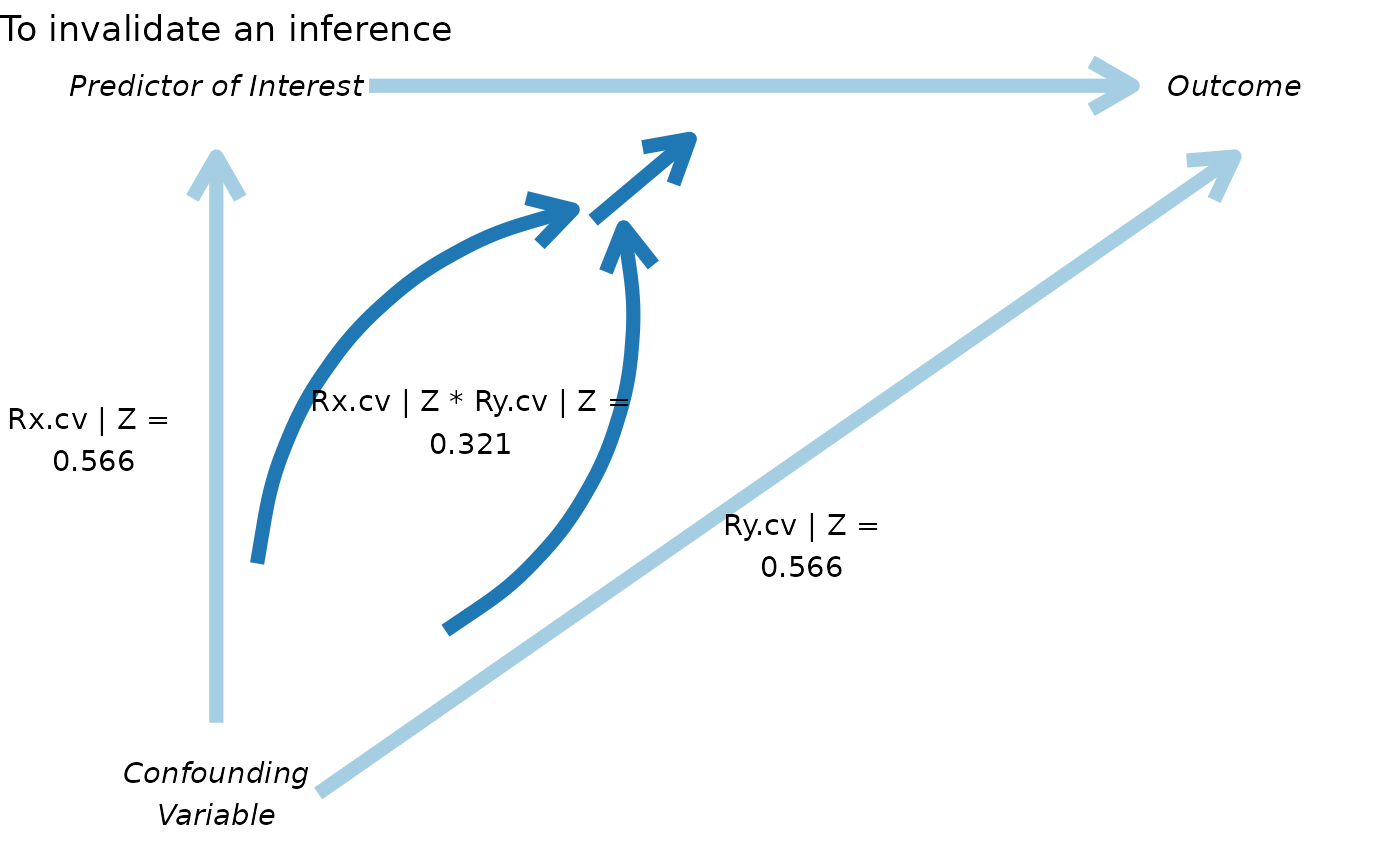
r_final: final correlation value given confounding variable (CV). Should be equal to critical_r
rxcv: unconditional \(corr(X,CV)\) necessary to nullify the inference for smallest impact
rycv: unconditional \(corr(Y,CV)\) necessary to nullify the inference for smallest impact
rxcvGz: \(corr(X,CV|Z)\) conditioning on all observed covariates
rycvGz: \(corr(Y,CV|Z)\) conditioning on all observed covariates
itcv: unconditional ITCV (uncond_rxcv * uncond_rycv)
itcvGz: conditional ITCV given all observed covariates
r2xz: \(R^2\) using all observed covariates to explain the predictor of interest (X)
r2yz: \(R^2\) using all observed covariates to explain the predictor of interest (Y)
beta_threshold: threshold for for estimated effect
beta_threshold_verify: verified threshold matching beta_threshold
perc_bias_to_change: percent bias to change inference
RIR_primary: Robustness of Inference to Replacement (RIR)
RIR_supplemental: RIR for an extra row or column that is needed to nullify the inference
RIR_perc: RIR as % of total sample (for linear regression) or as % of data points in the cell where replacement takes place (for logistic and 2 by 2 table)
Fig_ITCV: ITCV plot object
Fig_RIR: RIR threshold plot object

COP for linear model

delta*: delta calculated using Oster’s unrestricted estimator
delta*restricted: delta calculated using Oster’s restricted estimator
delta_exact: delta calculated using correlation-based approach
delta_pctbias: percent bias when comparing delta* to delta_exact
var(Y): variance of the dependent variable (\(\sigma_Y^2\))
var(X): variance of the independent variable (\(\sigma_X^2\))
var(CV): variance of the confounding variable (\(\sigma_{CV}^2\))
cor_oster: correlation matrix implied by delta*
cor_exact: correlation matrix implied by delta_exact
eff_x_M3_oster: effect estimate for X under the Oster‑PSE variant
eff_x_M3: effect estimate for X under the PSE adjustment
Table: formatted results table
Figure: COP diagnostic plot

PSE for linear model

corr(X,CV|Z): correlation between X and CV conditional on Z
corr(Y,CV|Z): correlation between Y and CV conditional on Z
corr(X,CV): correlation between X and CV
corr(Y,CV): correlation between X and CV
covariance matrix: covariance matrix among Y, X, Z, and CV under the PSE adjustment
eff_M3: estimated unstandardized regression coefficient for X in M3 under the PSE adjustment
se_M3: standard error of that coefficient in M3 under the PSE adjustment
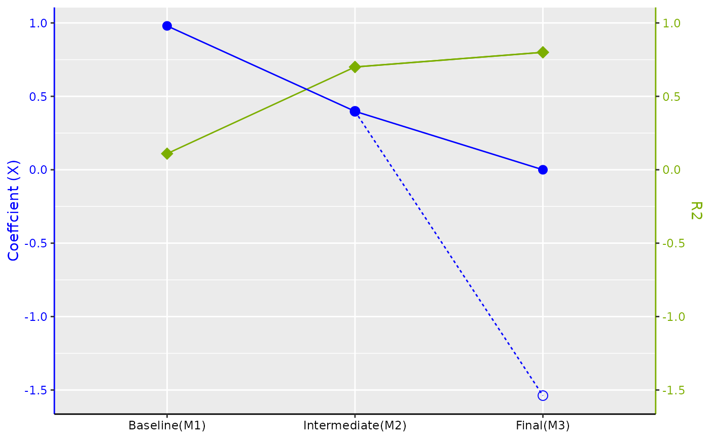
Table: matrix summarizing key statistics from three nested regression models (M1, M2, M3)

RIR for logistic model

RIR_primary: Robustness of Inference to Replacement (RIR)
RIR_supplemental: RIR for an extra row or column that is needed to nullify the inference
RIR_perc: RIR as % of data points in the cell where replacement takes place
fragility_primary: Fragility; the number of switches (e.g., treatment success to treatment failure) to nullify the inference
fragility_supplemental: Fragility for an extra row or column that is needed to nullify the inference
starting_table: observed (implied) 2 by 2 table before replacement and switching
final_table: the 2 by 2 table after replacement and switching
user_SE: user-entered standard error
analysis_SE: the standard error used to generate a plausible 2 by 2 table
needtworows: indicator whether extra switches were needed

RIR for 2×2 table model

RIR_primary: Robustness of Inference to Replacement (RIR)
RIR_supplemental: RIR for an extra row or column that is needed to nullify the inference
RIR_perc: RIR as % of data points in the cell where replacement takes place
fragility_primary: Fragility; the number of switches (e.g., treatment success to treatment failure) to nullify the inference
fragility_supplemental: Fragility for an extra row or column that is needed to nullify the inference
starting_table: observed 2 by 2 table before replacement and switching
final_table: the 2 by 2 table after replacement and switching
needtworows: indicator whether extra switches were needed

Examples

## Linear models
pkonfound(2, .4, 100, 3)
#> Robustness of Inference to Replacement (RIR):
#> RIR = 60
#> 
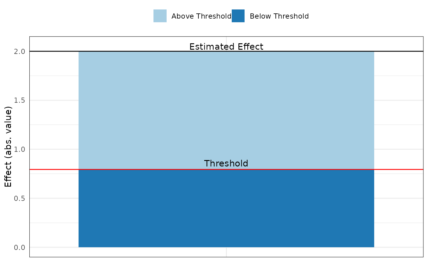
#> To nullify the inference of an effect using the threshold of 0.794 for
#> statistical significance (with null hypothesis = 0 and alpha = 0.05), 60.295%
#> of the estimate of 2 would have to be due to bias. This implies that to
#> nullify the inference one would expect to have to replace 60 (60.295%)
#> observations with data points for which the effect is 0 (RIR = 60).
#> 
#> See Frank et al. (2013) for a description of the method.
#> 
#> Citation: Frank, K.A., Maroulis, S., Duong, M., and Kelcey, B. (2013).
#> What would it take to change an inference?
#> Using Rubin's causal model to interpret the robustness of causal inferences.
#> Education, Evaluation and Policy Analysis, 35 437-460.
#> 
#> Accuracy of results increases with the number of decimals reported.
#> 
#> For other forms of output, run
#>           ?pkonfound and inspect the to_return argument
#> For models fit in R, consider use of konfound().
pkonfound(-2.2, .65, 200, 3)
#> Robustness of Inference to Replacement (RIR):
#> RIR = 83
#> 
#> To nullify the inference of an effect using the threshold of -1.282 for
#> statistical significance (with null hypothesis = 0 and alpha = 0.05), 41.73%
#> of the estimate of -2.2 would have to be due to bias. This implies that to
#> nullify the inference one would expect to have to replace 83 (41.73%)
#> observations with data points for which the effect is 0 (RIR = 83).
#> 
#> See Frank et al. (2013) for a description of the method.
#> 
#> Citation: Frank, K.A., Maroulis, S., Duong, M., and Kelcey, B. (2013).
#> What would it take to change an inference?
#> Using Rubin's causal model to interpret the robustness of causal inferences.
#> Education, Evaluation and Policy Analysis, 35 437-460.
#> 
#> Accuracy of results increases with the number of decimals reported.
#> 
#> For other forms of output, run
#>           ?pkonfound and inspect the to_return argument
#> For models fit in R, consider use of konfound().
pkonfound(.5, 3, 200, 3)
#> Robustness of Inference to Replacement (RIR):
#> RIR = 183
#> 
#> The estimated effect is 0.5. The threshold value for statistical significance
#> is 5.917 (with null hypothesis = 0 and alpha = 0.05). To reach that threshold,
#> 91.549% of the estimate of 0.5 would have to be due to bias. This implies to sustain
#> an inference one would expect to have to replace 183 (91.549%) observations with
#> effect of 0 with data points with effect of 5.917 (RIR = 183).
#> 
#> See Frank et al. (2013) for a description of the method.
#> 
#> Citation: Frank, K.A., Maroulis, S., Duong, M., and Kelcey, B. (2013).
#> What would it take to change an inference?
#> Using Rubin's causal model to interpret the robustness of causal inferences.
#> Education, Evaluation and Policy Analysis, 35 437-460.
#> 
#> Accuracy of results increases with the number of decimals reported.
#> 
#> For other forms of output, run
#>           ?pkonfound and inspect the to_return argument
#> For models fit in R, consider use of konfound().
# using a confidence interval
pkonfound(upper_bound = 3, lower_bound = 1, n_obs = 100, n_covariates = 3)   
#> Robustness of Inference to Replacement (RIR):
#> RIR = 50
#> 
#> To nullify the inference of an effect using the threshold of 1 for
#> statistical significance (with null hypothesis = 0 and alpha = 0.05), 49.987%
#> of the estimate of 2 would have to be due to bias. This implies that to
#> nullify the inference one would expect to have to replace 50 (49.987%)
#> observations with data points for which the effect is 0 (RIR = 50).
#> 
#> See Frank et al. (2013) for a description of the method.
#> 
#> Citation: Frank, K.A., Maroulis, S., Duong, M., and Kelcey, B. (2013).
#> What would it take to change an inference?
#> Using Rubin's causal model to interpret the robustness of causal inferences.
#> Education, Evaluation and Policy Analysis, 35 437-460.
#> 
#> Accuracy of results increases with the number of decimals reported.
#> 
#> For other forms of output, run
#>           ?pkonfound and inspect the to_return argument
#> For models fit in R, consider use of konfound().

## Plot examples
pkonfound(2, .4, 100, 3, to_return = "thresh_plot")

pkonfound(2, .4, 100, 3, to_return = "corr_plot")


## Logistic regression model example
pkonfound(-0.2, 0.103, 20888, 3, n_treat = 17888, model_type = "logistic")
#> Robustness of Inference to Replacement (RIR):
#> RIR = 2
#> Fragility = 1
#> 
#> You entered: log odds = -0.200, SE = 0.103, with p-value = 0.052. 
#> The table implied by the parameter estimates and sample sizes you entered:
#> 
#> Implied Table:
#>            Fail Success Success_Rate
#> Control    2882     118        3.93%
#> Treatment 17308     580        3.24%
#> Total     20190     698        3.34%
#> 
#> Values in the table have been rounded to the nearest integer. This may cause 
#> a small change to the estimated effect for the table.
#> 
#> To sustain an inference that the effect is different from 0 (alpha = 0.050), one would
#> need to transfer 1 data points from treatment success to treatment failure (Fragility = 1).
#> This is equivalent to replacing 2 (0.345%) treatment success data points with data points 
#> for which the probability of failure in the control group (96.067%) applies (RIR = 2). 
#> 
#> Note that RIR = Fragility/P(destination) = 1/0.961 ~ 2.
#> 
#> The transfer of 1 data points yields the following table:
#> 
#> Transfer Table:
#>            Fail Success Success_Rate
#> Control    2882     118        3.93%
#> Treatment 17309     579        3.24%
#> Total     20191     697        3.34%
#> 
#> The log odds (estimated effect) = -0.202, SE = 0.103, p-value = 0.050.
#> This p-value is based on t = estimated effect/standard error
#> 
#> Benchmarking RIR for Logistic Regression (Beta Version)
#> The treatment is not statistically significant in the implied table and would also not be
#> statistically significant in the raw table (before covariates were added). In this scenario, we
#> do not yet have a clear interpretation of the benchmark and therefore the benchmark calculation
#> is not reported.
#> 
#> See Frank et al. (2021) for a description of the methods.
#> 
#> *Frank, K. A., *Lin, Q., *Maroulis, S., *Mueller, A. S., Xu, R., Rosenberg, J. M., ... & Zhang, L. (2021).
#> Hypothetical case replacement can be used to quantify the robustness of trial results. Journal of Clinical
#> Epidemiology, 134, 150-159.
#> *authors are listed alphabetically.
#> 
#> Accuracy of results increases with the number of decimals entered.
#> 
#> For other forms of output, run
#>           ?pkonfound and inspect the to_return argument
#> For models fit in R, consider use of konfound().

## 2x2 table examples
pkonfound(a = 35, b = 17, c = 17, d = 38)
#> Robustness of Inference to Replacement (RIR):
#> RIR = 14
#> Fragility = 9
#> 
#> This function calculates the number of data points that would have to be replaced with
#> zero effect data points (RIR) to nullify the inference made about the association
#> between the rows and columns in a 2x2 table.
#> One can also interpret this as switches (Fragility) from one cell to another, such as from the
#> treatment success cell to the treatment failure cell.
#> 
#> To nullify the inference that the effect is different from 0 (alpha = 0.05),
#> one would need to transfer 9 data points from treatment success to treatment failure as shown,
#> from the User-entered Table to the Transfer Table (Fragility = 9).
#> This is equivalent to replacing 14 (36.842%) treatment success data points with data points
#> for which the probability of failure in the control group (67.308%) applies (RIR = 14). 
#> 
#> RIR = Fragility/P(destination)
#> 
#> For the User-entered Table, the estimated odds ratio is 4.530, with p-value of 0.000:
#> User-entered Table:
#>           Fail Success Success_Rate
#> Control     35      17       32.69%
#> Treatment   17      38       69.09%
#> Total       52      55       51.40%
#> 
#> For the Transfer Table, the estimated odds ratio is 2.278, with p-value of 0.051:
#> Transfer Table:
#>           Fail Success Success_Rate
#> Control     35      17       32.69%
#> Treatment   26      29       52.73%
#> Total       61      46       42.99%
#> 
#> See Frank et al. (2021) for a description of the methods.
#> 
#> *Frank, K. A., *Lin, Q., *Maroulis, S., *Mueller, A. S., Xu, R., Rosenberg, J. M., ... & Zhang, L. (2021).
#> Hypothetical case replacement can be used to quantify the robustness of trial results. Journal of Clinical
#> Epidemiology, 134, 150-159.
#> *authors are listed alphabetically.
#> 
#> For other forms of output, run
#>           ?pkonfound and inspect the to_return argument
#> For models fit in R, consider use of konfound().
pkonfound(a = 35, b = 17, c = 17, d = 38, alpha = 0.01)
#> Robustness of Inference to Replacement (RIR):
#> RIR = 9
#> Fragility = 6
#> 
#> This function calculates the number of data points that would have to be replaced with
#> zero effect data points (RIR) to nullify the inference made about the association
#> between the rows and columns in a 2x2 table.
#> One can also interpret this as switches (Fragility) from one cell to another, such as from the
#> treatment success cell to the treatment failure cell.
#> 
#> To nullify the inference that the effect is different from 0 (alpha = 0.01),
#> one would need to transfer 6 data points from treatment success to treatment failure as shown,
#> from the User-entered Table to the Transfer Table (Fragility = 6).
#> This is equivalent to replacing 9 (23.684%) treatment success data points with data points
#> for which the probability of failure in the control group (67.308%) applies (RIR = 9). 
#> 
#> RIR = Fragility/P(destination)
#> 
#> For the User-entered Table, the estimated odds ratio is 4.530, with p-value of 0.000:
#> User-entered Table:
#>           Fail Success Success_Rate
#> Control     35      17       32.69%
#> Treatment   17      38       69.09%
#> Total       52      55       51.40%
#> 
#> For the Transfer Table, the estimated odds ratio is 2.835, with p-value of 0.011:
#> Transfer Table:
#>           Fail Success Success_Rate
#> Control     35      17       32.69%
#> Treatment   23      32       58.18%
#> Total       58      49       45.79%
#> 
#> See Frank et al. (2021) for a description of the methods.
#> 
#> *Frank, K. A., *Lin, Q., *Maroulis, S., *Mueller, A. S., Xu, R., Rosenberg, J. M., ... & Zhang, L. (2021).
#> Hypothetical case replacement can be used to quantify the robustness of trial results. Journal of Clinical
#> Epidemiology, 134, 150-159.
#> *authors are listed alphabetically.
#> 
#> For other forms of output, run
#>           ?pkonfound and inspect the to_return argument
#> For models fit in R, consider use of konfound().
pkonfound(a = 35, b = 17, c = 17, d = 38, alpha = 0.01, switch_trm = FALSE)
#> Robustness of Inference to Replacement (RIR):
#> RIR = 19
#> Fragility = 6
#> 
#> This function calculates the number of data points that would have to be replaced with
#> zero effect data points (RIR) to nullify the inference made about the association
#> between the rows and columns in a 2x2 table.
#> One can also interpret this as switches (Fragility) from one cell to another, such as from the
#> treatment success cell to the treatment failure cell.
#> 
#> To nullify the inference that the effect is different from 0 (alpha = 0.01),
#> one would need to transfer 6 data points from control failure to control success as shown,
#> from the User-entered Table to the Transfer Table (Fragility = 6).
#> This is equivalent to replacing 19 (54.286%) control failure data points with data points
#> for which the probability of success in the control group (32.692%) applies (RIR = 19). 
#> 
#> RIR = Fragility/P(destination)
#> 
#> For the User-entered Table, the estimated odds ratio is 4.530, with p-value of 0.000:
#> User-entered Table:
#>           Fail Success Success_Rate
#> Control     35      17       32.69%
#> Treatment   17      38       69.09%
#> Total       52      55       51.40%
#> 
#> For the Transfer Table, the estimated odds ratio is 2.790, with p-value of 0.012:
#> Transfer Table:
#>           Fail Success Success_Rate
#> Control     29      23       44.23%
#> Treatment   17      38       69.09%
#> Total       46      61       57.01%
#> 
#> See Frank et al. (2021) for a description of the methods.
#> 
#> *Frank, K. A., *Lin, Q., *Maroulis, S., *Mueller, A. S., Xu, R., Rosenberg, J. M., ... & Zhang, L. (2021).
#> Hypothetical case replacement can be used to quantify the robustness of trial results. Journal of Clinical
#> Epidemiology, 134, 150-159.
#> *authors are listed alphabetically.
#> 
#> For other forms of output, run
#>           ?pkonfound and inspect the to_return argument
#> For models fit in R, consider use of konfound().
pkonfound(a = 35, b = 17, c = 17, d = 38, test = "chisq")
#> Robustness of Inference to Replacement (RIR):
#> RIR = 15
#> Fragility = 10
#> 
#> This function calculates the number of data points that would have to be replaced with
#> zero effect data points (RIR) to nullify the inference made about the association
#> between the rows and columns in a 2x2 table.
#> One can also interpret this as switches (Fragility) from one cell to another, such as from the
#> treatment success cell to the treatment failure cell.
#> 
#> To nullify the inference that the effect is different from 0 (alpha = 0.05),
#> one would need to transfer 10 data points from treatment success to treatment failure as shown,
#> from the User-entered Table to the Transfer Table (Fragility = 10).
#> This is equivalent to replacing 15 (39.474%) treatment success data points with data points
#> for which the probability of failure in the control group (67.308%) applies (RIR = 15). 
#> 
#> RIR = Fragility/P(destination)
#> 
#> For the User-entered Table, the Pearson's chi square is 14.176, with p-value of 0.000:
#> User-entered Table:
#>           Fail Success Success_Rate
#> Control     35      17       32.69%
#> Treatment   17      38       69.09%
#> Total       52      55       51.40%
#> 
#> For the Transfer Table, the Pearson's chi square is 3.640, with p-value of 0.056:
#> Transfer Table:
#>           Fail Success Success_Rate
#> Control     35      17       32.69%
#> Treatment   27      28       50.91%
#> Total       62      45       42.06%
#> 
#> See Frank et al. (2021) for a description of the methods.
#> 
#> *Frank, K. A., *Lin, Q., *Maroulis, S., *Mueller, A. S., Xu, R., Rosenberg, J. M., ... & Zhang, L. (2021).
#> Hypothetical case replacement can be used to quantify the robustness of trial results. Journal of Clinical
#> Epidemiology, 134, 150-159.
#> *authors are listed alphabetically.
#> 
#> For other forms of output, run
#>           ?pkonfound and inspect the to_return argument
#> For models fit in R, consider use of konfound().

## Advanced examples
# Calculating unconditional ITCV and benchmark correlation for ITCV
pkonfound(est_eff = .5, std_err = .056, n_obs = 6174, sdx = 0.22, sdy = 1, R2 = .3,
          index = "IT", to_return = "print")
#> Impact Threshold for a Confounding Variable (ITCV):
#> Unconditional ITCV:
#> The minimum impact of an omitted variable to nullify an inference for
#> a null hypothesis of an effect of 0 (nu) is based on a correlation of 0.253
#> with the outcome and 0.26 with the predictor of interest (BEFORE conditioning
#> on observed covariates; signs are interchangeable if they are different).
#> This is based on a threshold effect of 0.025 for statistical significance (alpha = 0.05).
#> 
#> Correspondingly the UNCONDITIONAL impact of an omitted variable (as defined in Frank 2000) must be
#> 0.253 X 0.26 = 0.066 to nullify an inference for a null hypothesis of an effect of 0 (nu).
#> 
#> Conditional ITCV:
#> The minimum impact of an omitted variable to nullify an inference for
#> a null hypothesis of an effect of 0 (nu) is based on a correlation of 0.3
#> with the outcome and 0.3 with the predictor of interest (conditioning on all
#> observed covariates in the model; signs are interchangeable if they are different).
#> This is based on a threshold effect of 0.025 for statistical significance (alpha = 0.05).
#> 
#> Correspondingly the conditional impact of an omitted variable (as defined in Frank 2000) must be 
#> 0.3 X 0.3 = 0.09 to nullify an inference for a null hypothesis of an effect of 0 (nu).
#> 
#> Interpretation of Benchmark Correlations for ITCV:
#> Benchmark correlation product ('benchmark_corr_product') is Rxz*Ryz = 0.0735, showing
#> the association strength of all observed covariates Z with X and Y.
#> 
#> The ratio ('itcv_ratio_to_benchmark') is unconditional ITCV/Benchmark = 0.0657/0.0735 = 0.8936.
#> 
#> The larger the ratio the stronger must be the unobserved impact relative to the
#> impact of all observed covariates to nullify the inference. The larger the ratio
#> the more robust the inference.
#> 
#> If Z includes pretests or fixed effects, the benchmark may be inflated, making the ratio
#> unusually small. Interpret robustness cautiously in such cases.
#> 
#> See Frank (2000) for a description of the method.
#> 
#> Citation:
#> Frank, K. (2000). Impact of a confounding variable on the inference of a
#> regression coefficient. Sociological Methods and Research, 29 (2), 147-194
#> 
#> Accuracy of results increases with the number of decimals reported.
#> 
#> The ITCV analysis was originally derived for OLS standard errors. If the
#> standard errors reported in the table were not based on OLS, some caution
#> should be used to interpret the ITCV.
#> For other forms of output, run
#>           ?pkonfound and inspect the to_return argument
#> For models fit in R, consider use of konfound().
# Calculating delta* and delta_exact 
pkonfound(est_eff = .4, std_err = .1, n_obs = 290, sdx = 2, sdy = 6, R2 = .7,
         eff_thr = 0, FR2max = .8, index = "COP", to_return = "raw_output")
#> $`delta*`
#> [1] 3.668243
#> 
#> $`delta*restricted`
#> [1] 4.085172
#> 
#> $delta_exact
#> [1] 1.508536
#> 
#> $delta_pctbias
#> [1] 143.1658
#> 
#> $cor_oster
#>            Y         X         Z        CV
#> Y  1.0000000 0.3266139 0.8266047 0.2579193
#> X  0.3266139 1.0000000 0.2433792 0.8659296
#> Z  0.8266047 0.2433792 1.0000000 0.0000000
#> CV 0.2579193 0.8659296 0.0000000 1.0000000
#> 
#> $cor_exact
#>            Y         X         Z        CV
#> Y  1.0000000 0.3266139 0.8266047 0.3416500
#> X  0.3266139 1.0000000 0.2433792 0.3671463
#> Z  0.8266047 0.2433792 1.0000000 0.0000000
#> CV 0.3416500 0.3671463 0.0000000 1.0000000
#> 
#> $`var(Y)`
#> [1] 36
#> 
#> $`var(X)`
#> [1] 4
#> 
#> $`var(CV)`
#> [1] 1
#> 
#> $eff_x_M3_oster
#> [1] -1.538308
#> 
#> $eff_x_M3
#> [1] -1.114065e-16
#> 
#> $Table
#>                 M1:X    M2:X,Z M3(delta_exact):X,Z,CV M3(delta*):X,Z,CV
#> R2         0.1097571 0.7008711           8.006897e-01         0.8006897
#> coef_X     0.9798418 0.3980344          -1.114065e-16        -1.5383085
#> SE_X       0.1665047 0.0995086           8.775619e-02         0.1803006
#> std_coef_X 0.3266139 0.2297940           0.000000e+00        -0.5127695
#> t_X        5.8847685 4.0000000          -1.269500e-15        -8.5319081
#> coef_CV           NA        NA           2.049900e+00         4.2116492
#> SE_CV             NA        NA           1.702349e-01         0.3497584
#> t_CV              NA        NA           1.204159e+01        12.0415946
#> 
#> $Figure
#> Warning: Use of `figTable$coef_X` is discouraged.
#> ℹ Use `coef_X` instead.
#> Warning: Use of `figTable$ModelLabel` is discouraged.
#> ℹ Use `ModelLabel` instead.
#> Warning: Use of `figTable$ModelLabel` is discouraged.
#> ℹ Use `ModelLabel` instead.
#> Warning: Use of `figTable$ModelLabel` is discouraged.
#> ℹ Use `ModelLabel` instead.
#> Warning: Use of `figTable$coef_X` is discouraged.
#> ℹ Use `coef_X` instead.
#> Warning: Use of `figTable$ModelLabel` is discouraged.
#> ℹ Use `ModelLabel` instead.

#> 
# Calculating rxcv and rycv when preserving standard error
pkonfound(est_eff = .5, std_err = .056, n_obs = 6174, eff_thr = .1,
         sdx = 0.22, sdy = 1, R2 = .3, index = "PSE", to_return = "raw_output")
#> $`correlation between X and CV conditional on Z`
#> [1] 0.2479732
#> 
#> $`correlation between Y and CV conditional on Z`
#> [1] 0.3721927
#> 
#> $`correlation between X and CV`
#> [1] 0.2143707
#> 
#> $`correlation between Y and CV`
#> [1] 0.313404
#> 
#> $`covariance matrix`
#>             Y          X         Z         CV
#> Y  1.00000000 0.07773579 0.5394031 0.31340398
#> X  0.07773579 0.04840000 0.1105826 0.04716155
#> Z  0.53940306 0.11058258 1.0000000 0.00000000
#> CV 0.31340398 0.04716155 0.0000000 1.00000000
#> 
#> $eff_M3
#> [1] 0.09740386
#> 
#> $se_M3
#> [1] 0.05397058
#> 
#> $Table
#>                   M1:X      M2:X,Z   M3:X,Z,CV
#> R2          0.12499409  0.30011338  0.38959867
#> coef_X      1.60611143  0.50004052  0.09740386
#> SE_X        0.05411712  0.05598639  0.05397058
#> std_coef_X  0.35334452  0.11294102  0.02142885
#> t_X        29.67843530  8.93146515  1.80475837
#> coef_Z              NA  0.48410729  0.52863189
#> SE_Z                NA  0.01231701  0.01159750
#> t_Z                 NA 39.30397315 45.58155174
#> coef_CV             NA          NA  0.30881026
#> SE_CV               NA          NA  0.01026456
#> t_CV                NA          NA 30.08509668
#>